Chapter 4 Exercise 9.5

4.1 Load packages

Here is the R code to download the required packages for this exercise.

# install package manager 'pacman'
if (!require(pacman)){
  install.packages('pacman')
}

## Loading required package: pacman

# load packages needed for this exercise
library(pacman)
p_load(tidyverse,
       lctools, # to calculate Moran's I
       spdep, # to calculate geary's c
       geoR, # to compute variogram
       gridExtra, # to stack plots
       gstat, automap, # packages for variogram model selection
       sp # need a function called `coordinates`
       )

4.2 Data

This is equivalent to data step in SAS. Here, the data is imported from a file data.csv using the function read_csv. This function will download the file directly from here.

# Import data
a <- read_csv("https://raw.githubusercontent.com/luckymehra/epidem-exercises/master/data/ex9_5.csv")

## Parsed with column specification:
## cols(
##   COL = col_double(),
##   ROW = col_double(),
##   YI = col_double()
## )

# print the data
a

## # A tibble: 144 x 3
##      COL   ROW    YI
##    <dbl> <dbl> <dbl>
##  1     1     1     2
##  2     2     1     2
##  3     3     1     0
##  4     4     1     3
##  5     5     1     1
##  6     6     1     1
##  7     7     1     1
##  8     8     1     5
##  9     9     1    22
## 10    10     1    13
## # ... with 134 more rows

4.3 Autocorrelation statistics

# visualize the data
ggplot(data = a) +
  geom_point(mapping = aes(x = COL, y = ROW, size = YI, color = YI)) +
  ggtitle("Spatial Distribution of YI Observation") +
  theme(plot.title = element_text(hjust = 0.5))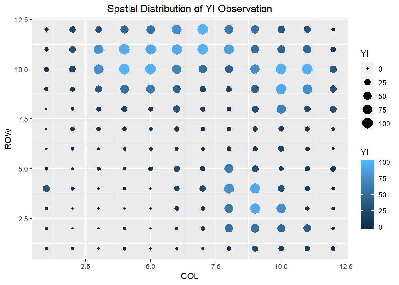

# calculate Moran's I
Coords <- a %>% 
  dplyr::select(COL, ROW)

mI <- moransI(Coords, Bandwidth = 1, a$YI)

# print Moran's I table
moran.table <- tribble(
  ~`Moran's I`, ~`Expected I`, ~`Z randomization`, ~`P value randomization`,
  #------------/--------------/-------------------/------------------------
  mI$Morans.I, mI$Expected.I,  mI$z.randomization, mI$p.value.randomization
  )

moran.table

## # A tibble: 1 x 4
##   `Moran's I` `Expected I` `Z randomization` `P value randomization`
##         <dbl>        <dbl>             <dbl>                   <dbl>
## 1       0.782     -0.00699              13.0                1.28e-38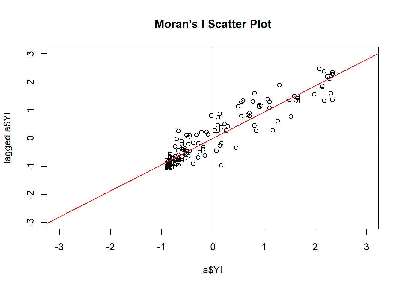

# create Moran's I scatter plot
l.moran <- l.moransI(Coords, Bandwidth = 1, a$YI)

# calculate geary's c
Coords_num <- coordinates(Coords)

# create an object of class 'nb' so that it can be used with function from packege `spdep`
Coords_nb <- knn2nb(knearneigh(Coords_num))

# create a 'listw' object for use in the function `geary.test`
coords_listw <- nb2listw(Coords_nb)

gearyC <- geary.test(a$YI, coords_listw, alternative = "two.sided")
gearyC

## 
##  Geary C test under randomisation
## 
## data:  a$YI 
## weights: coords_listw 
## 
## Geary C statistic standard deviate = 8.8657, p-value < 2.2e-16
## alternative hypothesis: two.sided
## sample estimates:
## Geary C statistic       Expectation          Variance 
##       0.235058006       1.000000000       0.007444457

4.4 First variogram

We will use the package geoR to construct empricial variogram, and then draw them using package ggplot2.

v1 <- variog(coords = Coords_num, data = a$YI, breaks = seq(0.5, 15.5),
             max.dist = 12)

## variog: computing omnidirectional variogram

# extract data from object v1 for plotting
v1_plot_data <- cbind(v1$u, v1$v, v1$n) %>% 
  as.data.frame() %>% 
  dplyr::rename(Distance = V1,
                Semivariance = V2,
                Pair_count = V3)

# in the table below, gamma is semivariance
v1_plot_data

##    Distance Semivariance Pair_count
## 1         1     311.7154        506
## 2         2     636.2074        680
## 3         3     818.7044        812
## 4         4     901.3218       1386
## 5         5     910.2773       1044
## 6         6     942.3219       1252
## 7         7     998.2290       1046
## 8         8    1131.2105       1012
## 9         9    1261.6817       1076
## 10       10    1219.6067        614
## 11       11    1166.5541        508
## 12       12     910.6250         80

# plot variogram
v1_plot_vario <- ggplot(data = v1_plot_data) +
  geom_point(mapping = aes(x = Distance, y = Semivariance)) +
  ggtitle("Empirical Semivariogram of YI") +
  theme(plot.title = element_text(hjust = 0.5))

# plot pair counts
v1_plot_pair_count <- ggplot(data = v1_plot_data) +
  geom_col(mapping = aes(x = Distance, y = Pair_count), width = 0.01, color = "blue")

# stack two plots
grid.arrange(v1_plot_vario, v1_plot_pair_count,
             ncol = 1, heights = c(3, 1))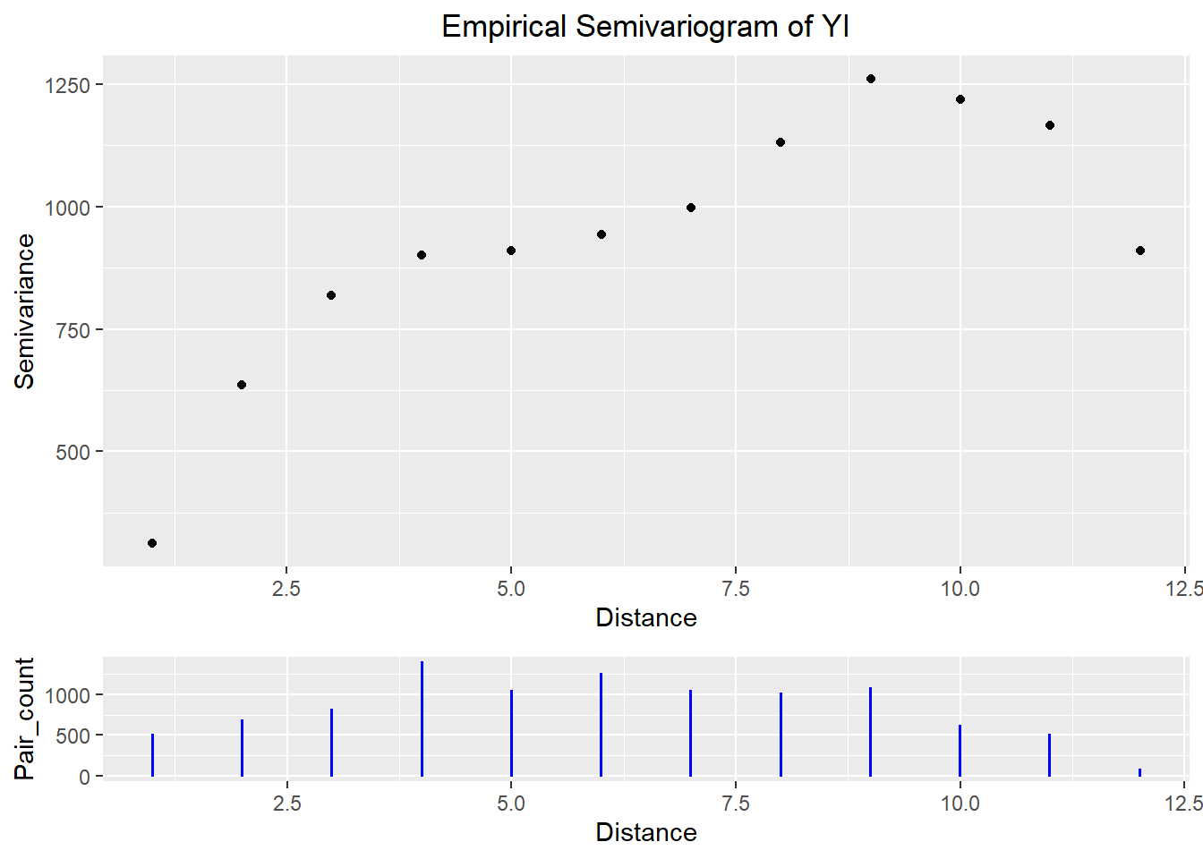

4.5 Second variogram

Plot robust and classical variogram together.

# fit robust variogram
v1_robust <- variog(coords = Coords_num, data = a$YI, breaks = seq(0.5, 15.5),
             max.dist = 12, estimator.type = "modulus")

## variog: computing omnidirectional variogram

# extract the data
v1_robust_data <- cbind(v1_robust$u, v1_robust$v, v1_robust$n) %>% 
  as.data.frame() %>% 
  dplyr::rename(Distance = V1,
                Semivariance = V2,
                Pair_count = V3)

# plot robust variogram
v1_robust_vario <- ggplot(data = v1_robust_data) +
  geom_point(mapping = aes(x = Distance, y = Semivariance)) +
  ggtitle("Empirical Semivariogram of YI - Robust estimation") +
  theme(plot.title = element_text(hjust = 0.5))

v1_robust_vario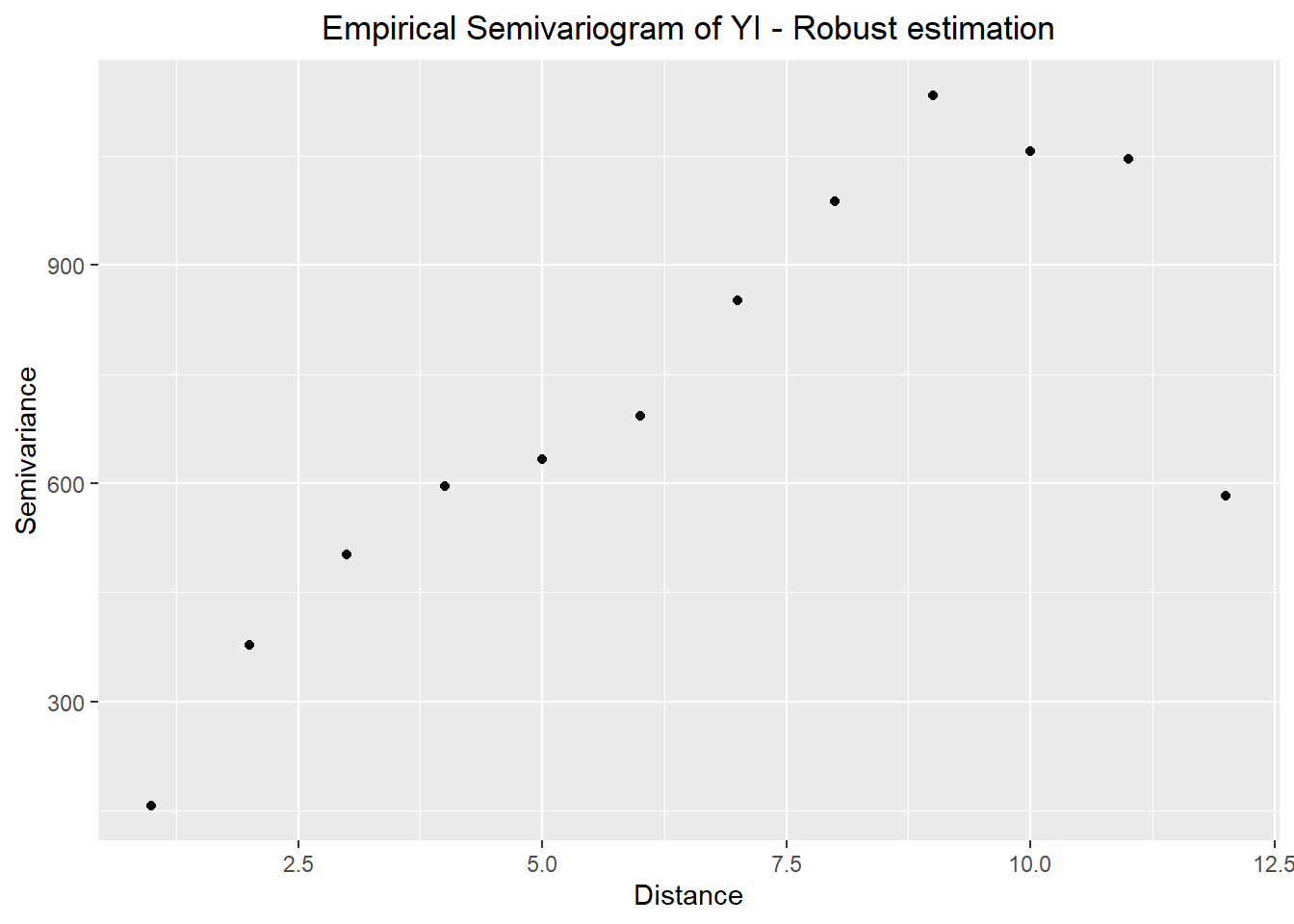

# combine robust and classical variogram  
var_comb <- v1_robust_data %>% 
  
  # combine robust and classical variogram datasets
  dplyr::rename(Semivariance_robust = Semivariance) %>% 
  bind_cols(dplyr::select(v1_plot_data, Semivariance)) %>% 
  gather(key = "Semivariance_type", value = "Semivariance", -c(Distance, Pair_count)) %>% 
  
  # plot
  ggplot() +
  geom_point(mapping = aes(x = Distance, y = Semivariance, color = Semivariance_type)) +
  ggtitle("Empirical Semivariogram for YI") +
  theme(plot.title = element_text(hjust = 0.5))

var_comb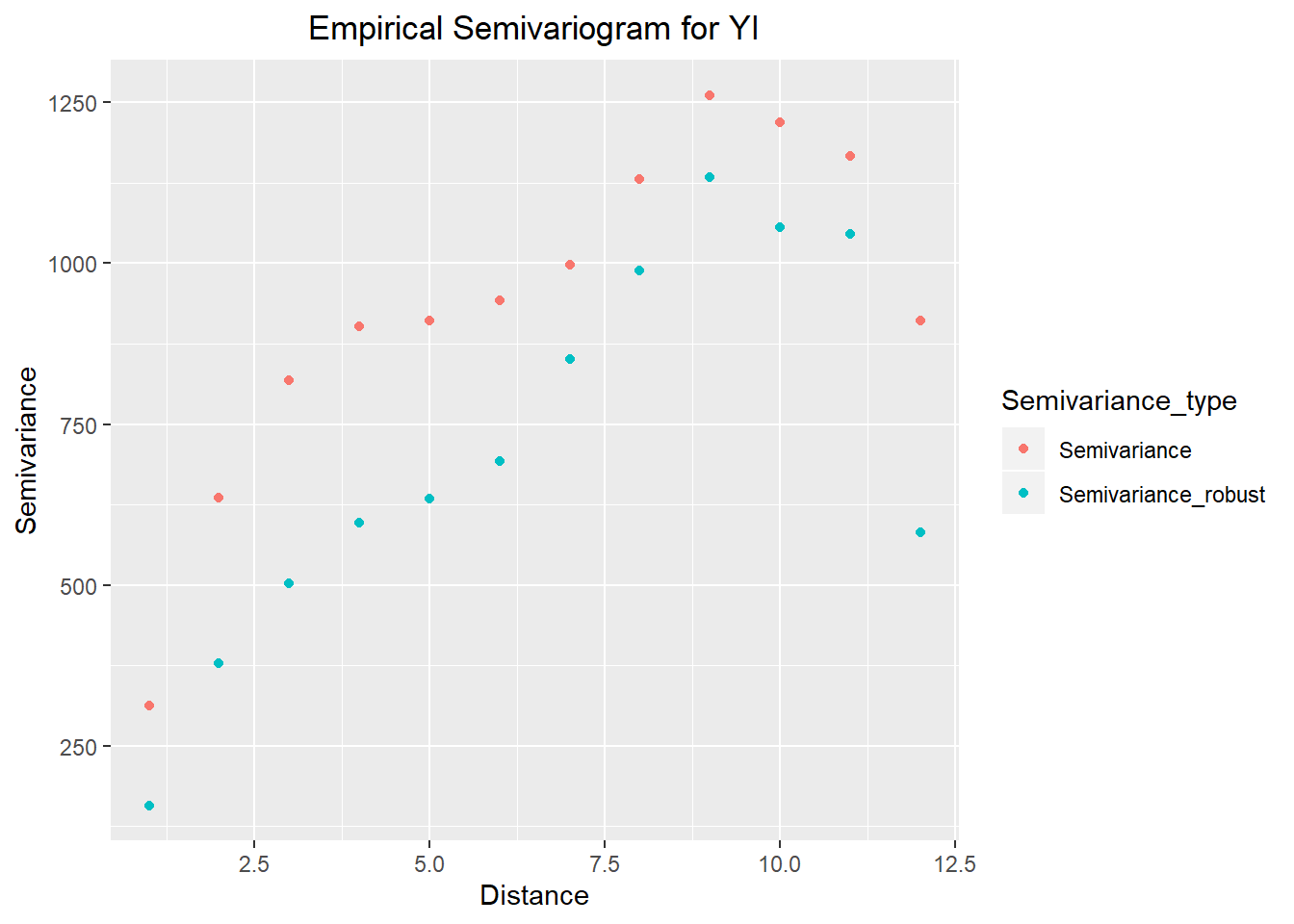

4.6 Variogram model selection

We will use the package gstat and automap for variogram model selection

# specify coordinates in the dataset
coordinates(a) = ~COL+ROW

# select the best model out of exponential, spherical, and gaussian  
autofitVariogram(YI ~ COL + ROW, a, model = c("Sph", "Exp", "Gau"), cutoff = 12)

## $exp_var
##     np     dist    gamma dir.hor dir.ver   id
## 1  264 1.000000 233.2400       0       0 var1
## 2  242 1.414214 388.5222       0       0 var1
## 3  680 2.152750 612.6985       0       0 var1
## 4  812 3.036881 756.8971       0       0 var1
## 5 1066 3.944315 783.1461       0       0 var1
## 6 1364 4.977586 742.6252       0       0 var1
## 
## $var_model
##   model    psill    range
## 1   Nug   0.0000 0.000000
## 2   Sph 782.9935 4.019145
## 
## $sserr
## [1] 1247749
## 
## attr(,"class")
## [1] "autofitVariogram" "list"

# fit empirical variogram
v_emp <- variogram(YI ~ COL + ROW, data = a, cutoff = 12)
v_emp

##      np      dist    gamma dir.hor dir.ver   id
## 1   506  1.198102 307.5054       0       0 var1
## 2   680  2.152750 612.6985       0       0 var1
## 3   812  3.036881 756.8971       0       0 var1
## 4   552  3.742751 784.3027       0       0 var1
## 5   834  4.280245 782.1560       0       0 var1
## 6  1044  5.132514 730.3844       0       0 var1
## 7  1028  6.012860 693.9058       0       0 var1
## 8   878  6.801676 675.9157       0       0 var1
## 9   836  7.525735 703.4337       0       0 var1
## 10  852  8.302717 728.0099       0       0 var1
## 11  792  9.194510 712.3311       0       0 var1
## 12  542 10.047104 621.2100       0       0 var1
## 13  452 10.826377 554.3985       0       0 var1
## 14  208 11.494850 599.2237       0       0 var1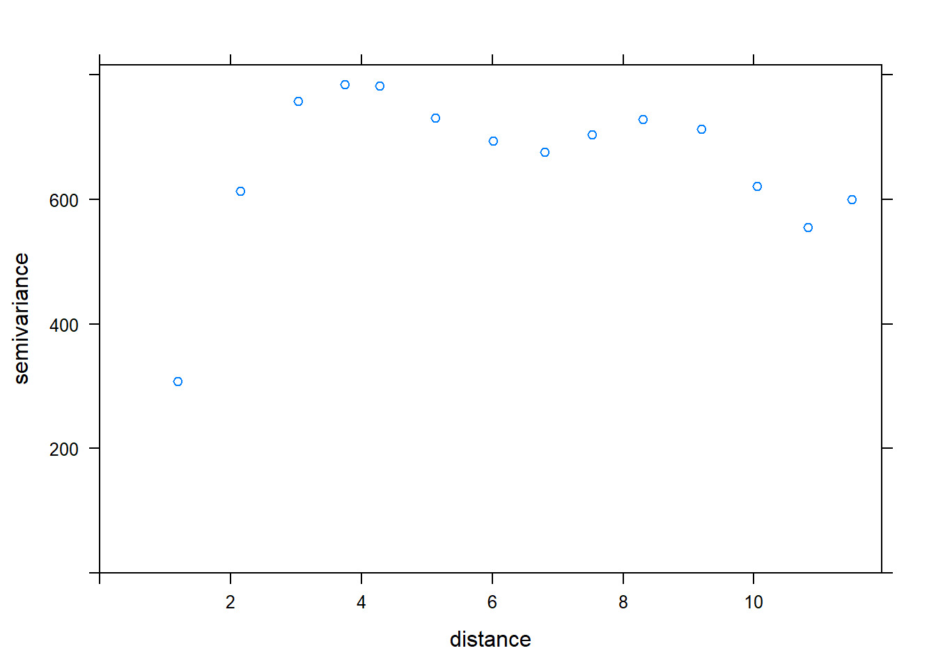

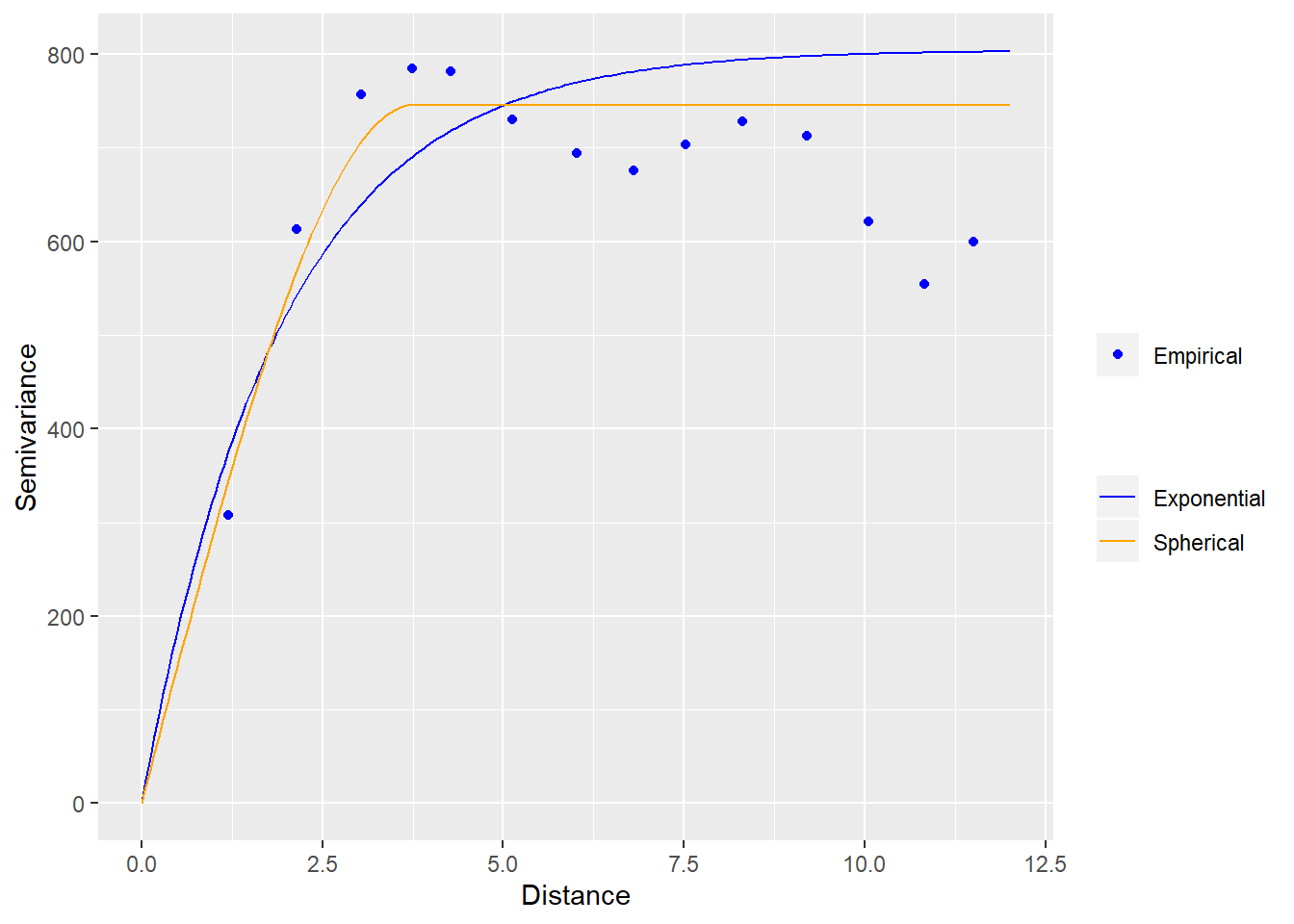
plot(v_emp)

# fit exponential variogram
v_exp <- fit.variogram(v_emp, vgm("Exp"))

# fit spherical and gaussian
v_sph <- fit.variogram(v_emp, vgm("Sph"))
v_sph

##   model    psill    range
## 1   Nug   0.0000 0.000000
## 2   Sph 745.8602 3.765221

v_gau <- fit.variogram(v_emp, vgm("Gau"))

## Warning in fit.variogram(v_emp, vgm("Gau")): No convergence after 200
## iterations: try different initial values?

# extract plotting data from fitted variograms
v_exp_line <- variogramLine(v_exp, maxdist = 12)
v_sph_line <- variogramLine(v_sph, maxdist = 12)
# v_gau_line <- variogramLine(v_gau, maxdist = 12)

# plot emprical and fitted variograms together  
# specify color for legends
legend_color <- c("Empirical" = "blue", "Exponential" = "blue",
                  "Spherical" = "orange")
ggplot(data = v_emp) +
  geom_point(mapping = aes(x = dist, y = gamma, fill = "Empirical"), color = "blue") +
  geom_line(data = v_exp_line, mapping = aes(x = dist, y = gamma, color = "Exponential")) +
  geom_line(data = v_sph_line, mapping = aes(x = dist, y = gamma, color = "Spherical")) +
  # geom_line(data = v_gau_line, mapping = aes(x = dist, y = gamma, color = "Gaussian")) +
  scale_color_manual(name = "", values = legend_color) +
  scale_fill_manual(name = "", values = legend_color) +
  labs(x = "Distance",
       y = "Semivariance")