Chapter 1 Exercise 1
1.1 Load packages
Here is the R code to download the required packages for this exercise.
## Loading required package: pacman1.2 Data
This is equivalent to the data step in SAS. Here, the data is imported from a file ex1.csv using the function read_csv. This function will download the data file direclty from here.
# Import data
a <- read_csv("data/ex1.csv") %>%
    # create a new variable `DIFF`
    mutate(DIFF = ESTIMATE - ACTUAL)
## Parsed with column specification:
## cols(
## TEST = col_character(),
## OBS = col_double(),
## ESTIMATE = col_double(),
## ACTUAL = col_double()
## )## # A tibble: 60 x 5
## TEST OBS ESTIMATE ACTUAL DIFF
## <chr> <dbl> <dbl> <dbl> <dbl>
## 1 BASELINE 1 2 7 -5
## 2 BASELINE 2 25 39 -14
## 3 BASELINE 3 35 49 -14
## 4 BASELINE 4 20 34 -14
## 5 BASELINE 5 5 8 -3
## 6 BASELINE 6 50 57 -7
## 7 BASELINE 7 5 14 -9
## 8 BASELINE 8 50 57 -7
## 9 BASELINE 9 60 73 -13
## 10 BASELINE 10 2 9 -7
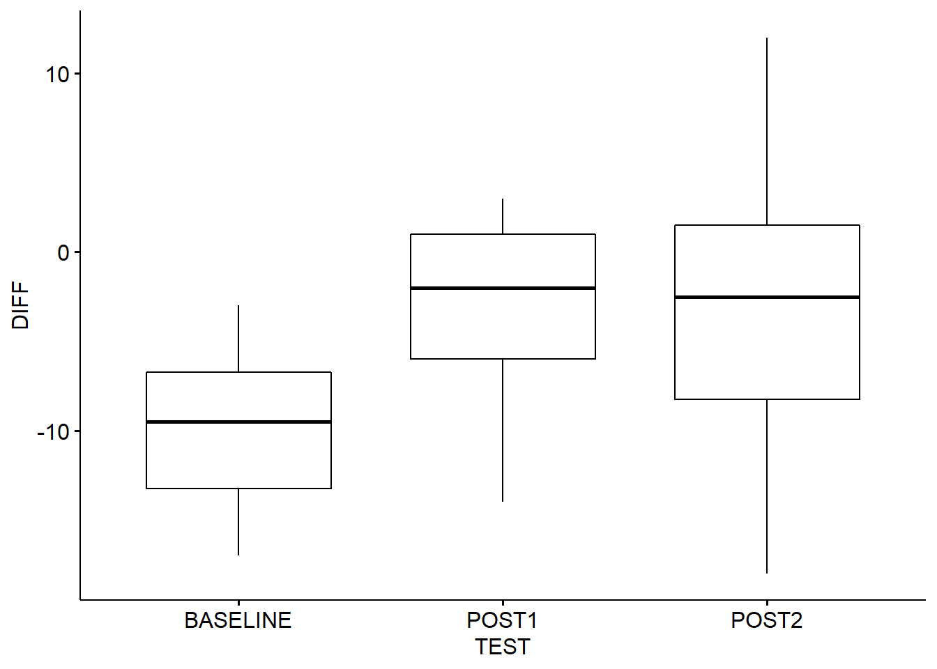
## # ... with 50 more rows1.3 Descriptive statistics
# use the describe() function to get an idea about different variables
sm_a <- a %>%
    group_by(TEST) %>%
    summarise_at(vars(DIFF),
                             list(~mean(., na.rm = TRUE),
                                     ~mode(.),
                                     ~median(., na.rm = TRUE),
                                     ~sd(., na.rm = TRUE),
                                     ~var(., na.rm = TRUE),
                                     ~IQR(., na.rm = TRUE),
                                     ~min(., na.rm = TRUE),
                                     ~max(., na.rm = TRUE),
                                     ~n(),
                                     ~skew(.),
                                     ~kurtosi(.)
                                     )) %>%
    mutate(CV = (sd/mean)*100,
                 std.err = sd/sqrt(n)) %>%
    ungroup()

sm_a
## # A tibble: 3 x 14
## TEST mean mode median sd var IQR min max n skew
## <chr> <dbl> <chr> <dbl> <dbl> <dbl> <dbl> <dbl> <dbl> <int> <dbl>
## 1 BASE~ -9.75 nume~ -9.5 4.17 17.4 6.5 -17 -3 20 -0.0599
## 2 POST1 -2.95 nume~ -2 4.43 19.6 7 -14 3 20 -0.804
## 3 POST2 -2.75 nume~ -2.5 8.82 77.8 9.75 -18 12 20 0.0162
## # ... with 3 more variables: kurtosi <dbl>, CV <dbl>, std.err <dbl>1.4 Create histogram, boxplot, and qqplot
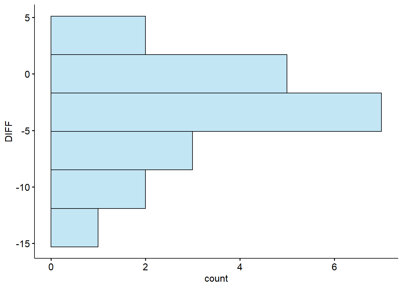
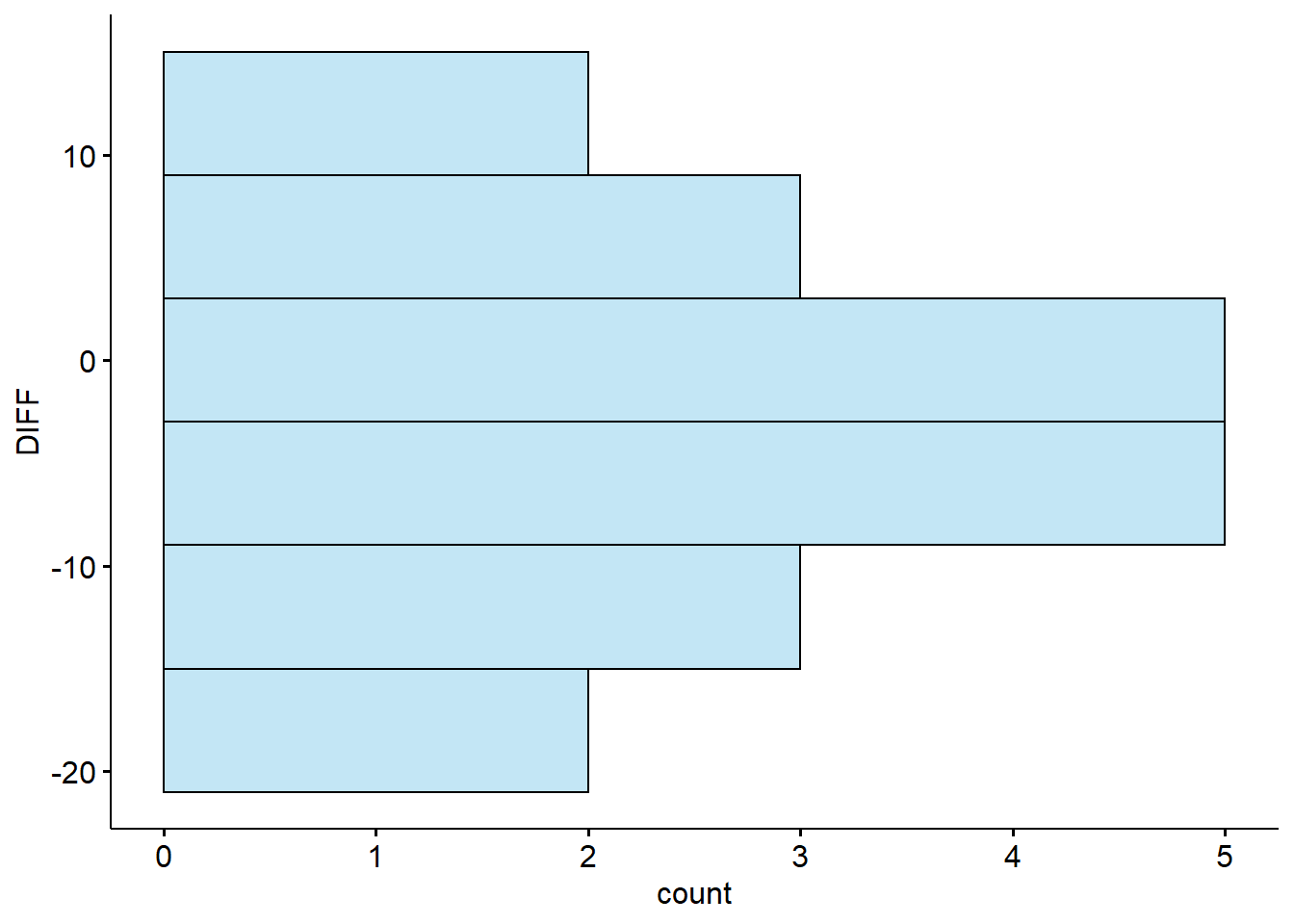
# histograms
create_hist <- function(test_id){
a %>%
    filter(TEST == {{test_id}}) %>%
    gghistogram("DIFF", bins = 6, fill = "skyblue") +
        coord_flip()
}

create_hist(unique(a$TEST)[1]) # BASELINE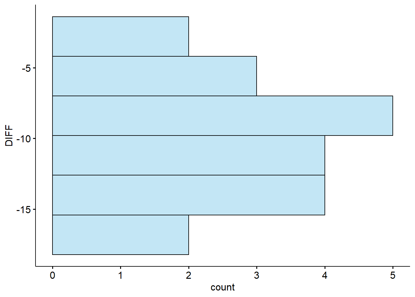
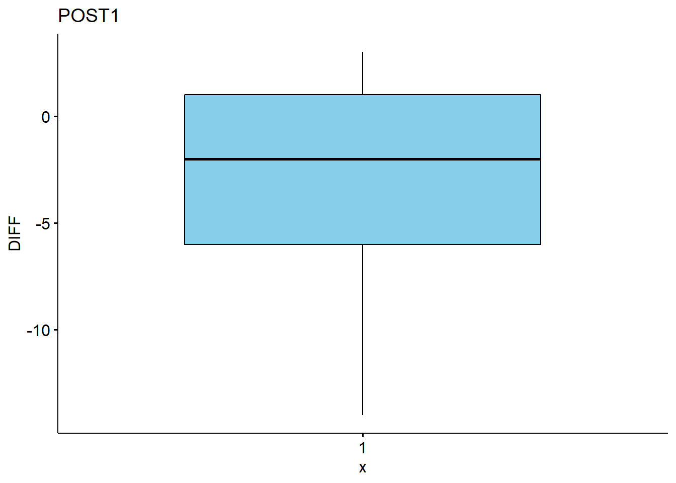
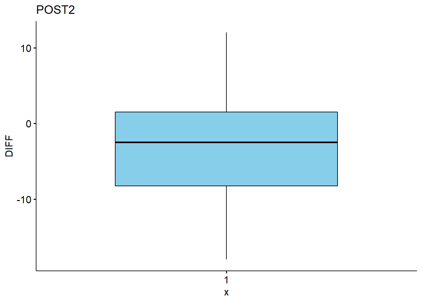
# boxplots
create_box <- function(test_id){
    a %>%
        filter(TEST == {{test_id}}) %>%
        ggboxplot(y = "DIFF", fill =  "skyblue",
                            main = {{test_id}})
}

create_box(unique(a$TEST)[1]) # BASELINE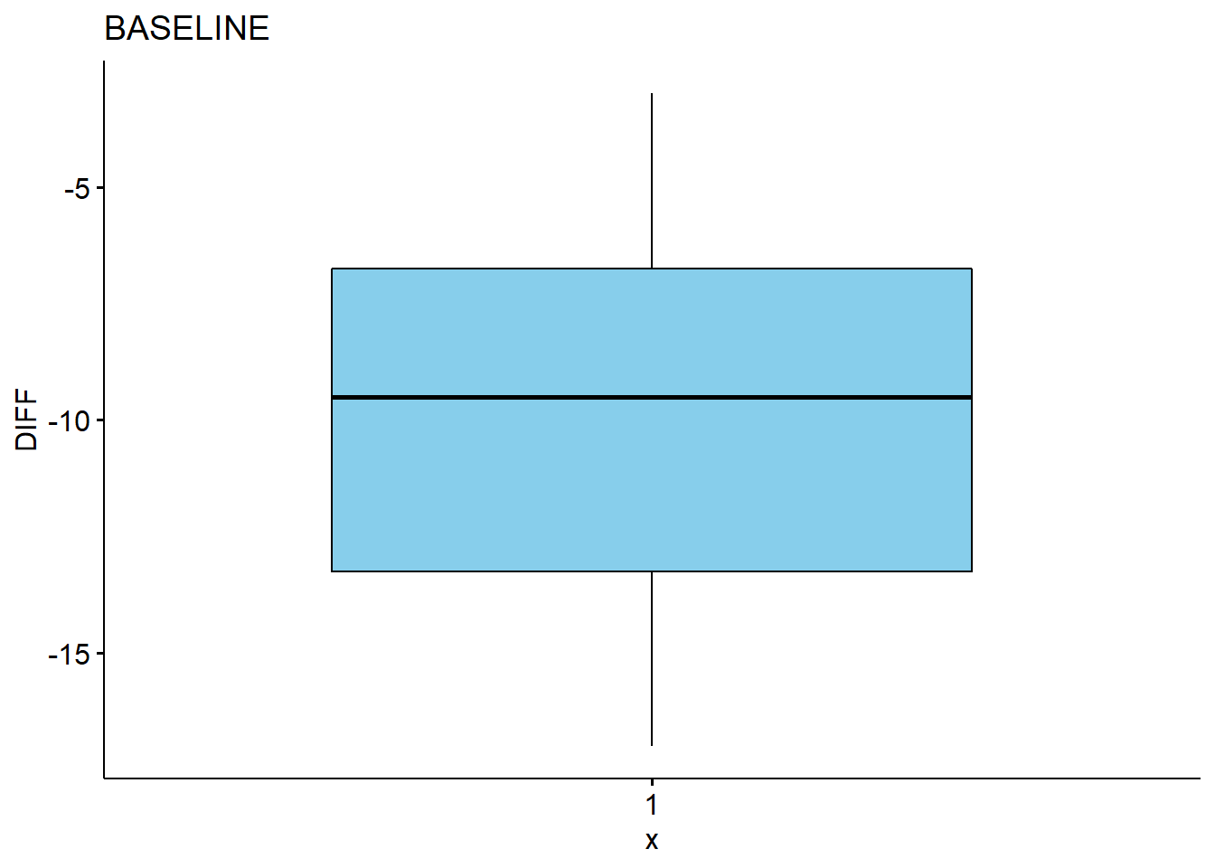
# qqplots
create_qq <- function(test_id){
a %>%
    filter(TEST == {{test_id}}) %>%
    ggqqplot("DIFF",
                     main = {{test_id}})
}

create_qq(unique(a$TEST)[1]) # BASELINE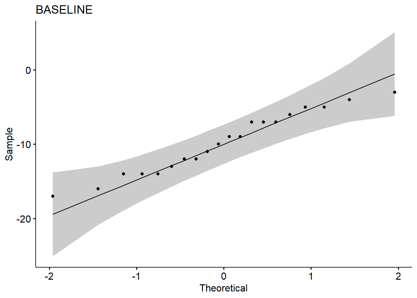
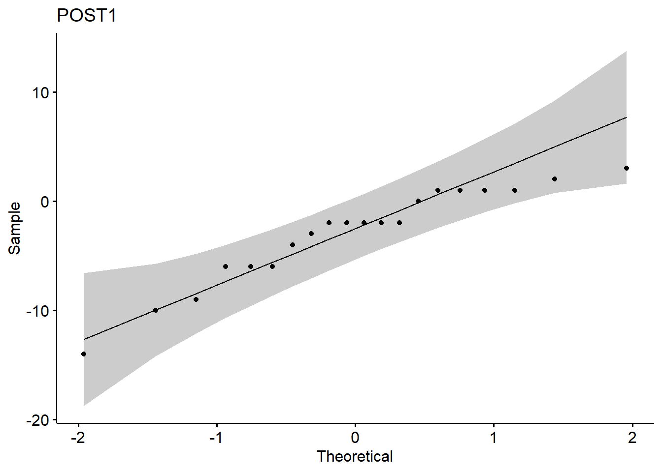
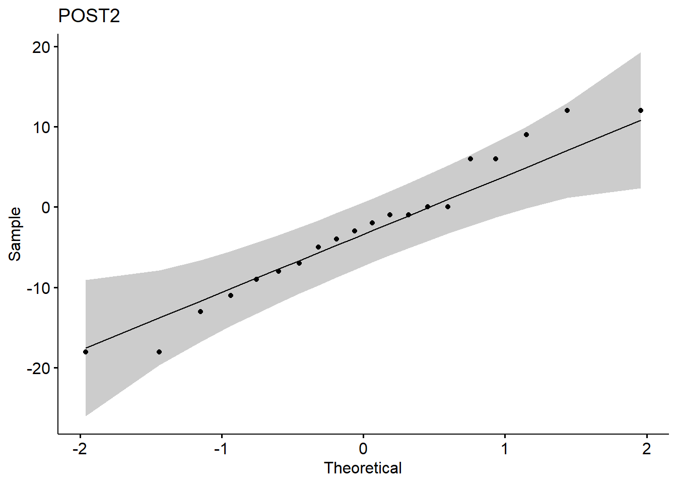
1.5 Normality test
##                     st.method st.statistic st.p.value
## W Shapiro-Wilk normality test    0.9783355  0.3622644
do_shp_test <- function(df){
st <- shapiro.test(df$DIFF)
data.frame(st$method, st$statistic, st$p.value)
}
a %>%
group_by(TEST) %>%
do(do_shp_test(.)) %>%
ungroup()## # A tibble: 3 x 4
## TEST st.method st.statistic st.p.value
## <chr> <fct> <dbl> <dbl>
## 1 BASELINE Shapiro-Wilk normality test 0.958 0.511
## 2 POST1 Shapiro-Wilk normality test 0.919 0.0958
## 3 POST2 Shapiro-Wilk normality test 0.965 0.6381.6 Linear regression
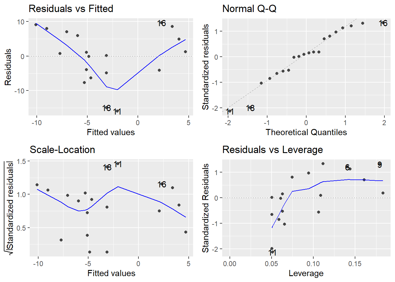
# fit linear regression by TEST
# Response: ESTIMATE
est_lm <- function(df){
    model <- lm(ESTIMATE ~ ACTUAL, data = df)

    # fit plot
    fit_plot <- ggplot(data = df, aes(x = ACTUAL, y = ESTIMATE)) +
        geom_point()+
        stat_smooth(method = "lm", col = "blue")

    return(list(summary(model), autoplot(model), fit_plot))
}

by(a, a$TEST, est_lm)
## a$TEST: BASELINE
## [[1]]
##
## Call:
## lm(formula = ESTIMATE ~ ACTUAL, data = df)
##
## Residuals:
## Min 1Q Median 3Q Max
## -7.3419 -3.0730 0.3805 3.2750 6.3549
##
## Coefficients:
## Estimate Std. Error t value Pr(>|t|)
## (Intercept) -9.1837 1.8107 -5.072 7.95e-05 ***
## ACTUAL 0.9852 0.0403 24.448 2.93e-15 ***
## ---
## Signif. codes: 0 '***' 0.001 '**' 0.01 '*' 0.05 '.' 0.1 ' ' 1
##
## Residual standard error: 4.264 on 18 degrees of freedom
## Multiple R-squared: 0.9708, Adjusted R-squared: 0.9691
## F-statistic: 597.7 on 1 and 18 DF, p-value: 2.933e-15
##
##
## [[2]]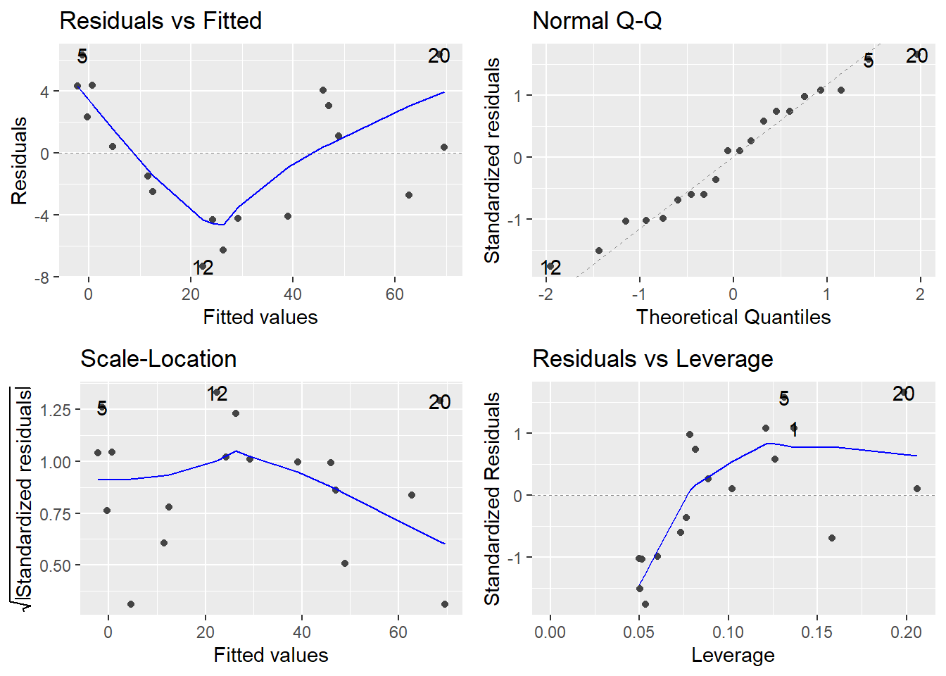
##
## [[3]]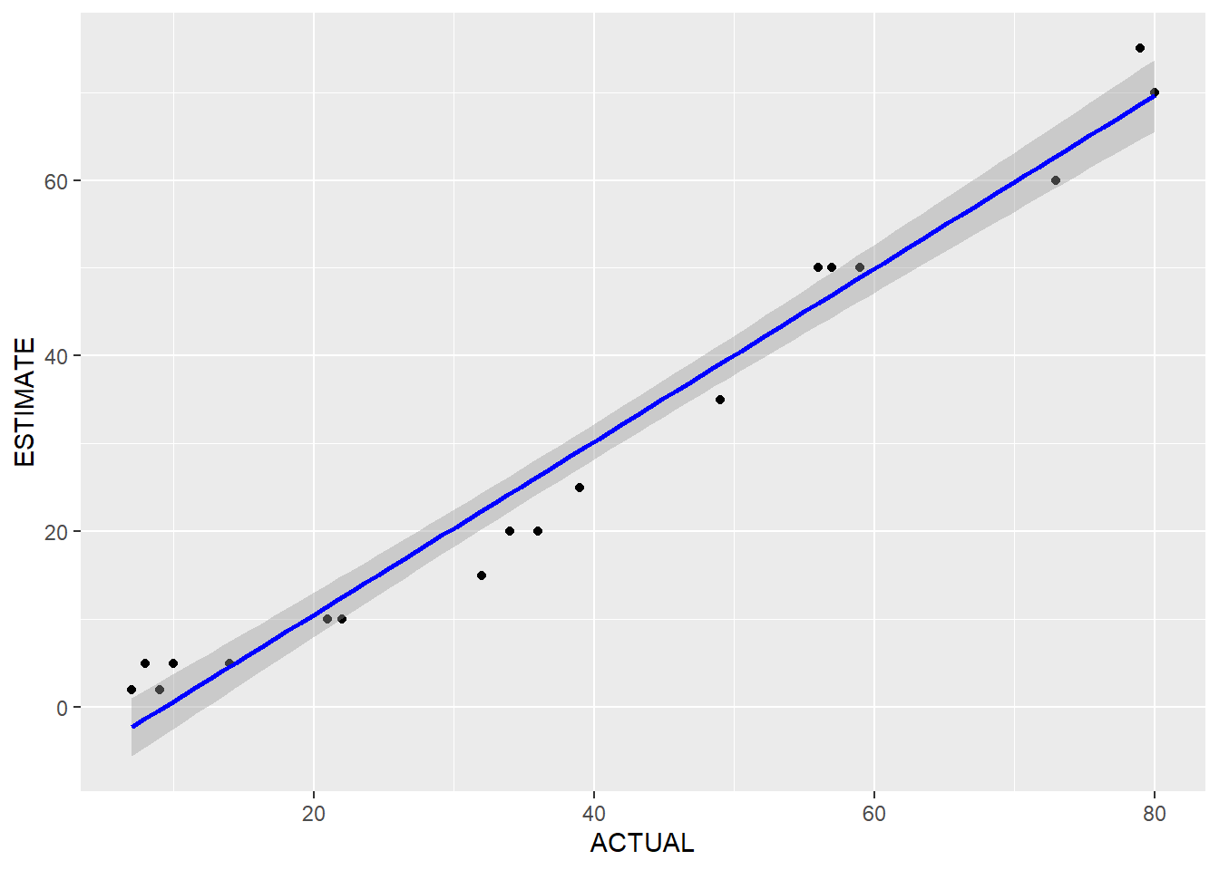
##
## --------------------------------------------------------
## a$TEST: POST1
## [[1]]
##
## Call:
## lm(formula = ESTIMATE ~ ACTUAL, data = df)
##
## Residuals:
##      Min       1Q   Median       3Q      Max
## -11.0323  -2.7663   0.6561   3.5244   6.3667
##
## Coefficients:
##             Estimate Std. Error t value Pr(>|t|)
## (Intercept)  -2.1033     1.9186  -1.096    0.287
## ACTUAL        0.9778     0.0427  22.901 9.18e-15 ***
## ---
## Signif. codes:  0 '***' 0.001 '**' 0.01 '*' 0.05 '.' 0.1 ' ' 1
##
## Residual standard error: 4.518 on 18 degrees of freedom
## Multiple R-squared:  0.9668, Adjusted R-squared:  0.965
## F-statistic: 524.5 on 1 and 18 DF,  p-value: 9.183e-15
##
##
## [[2]]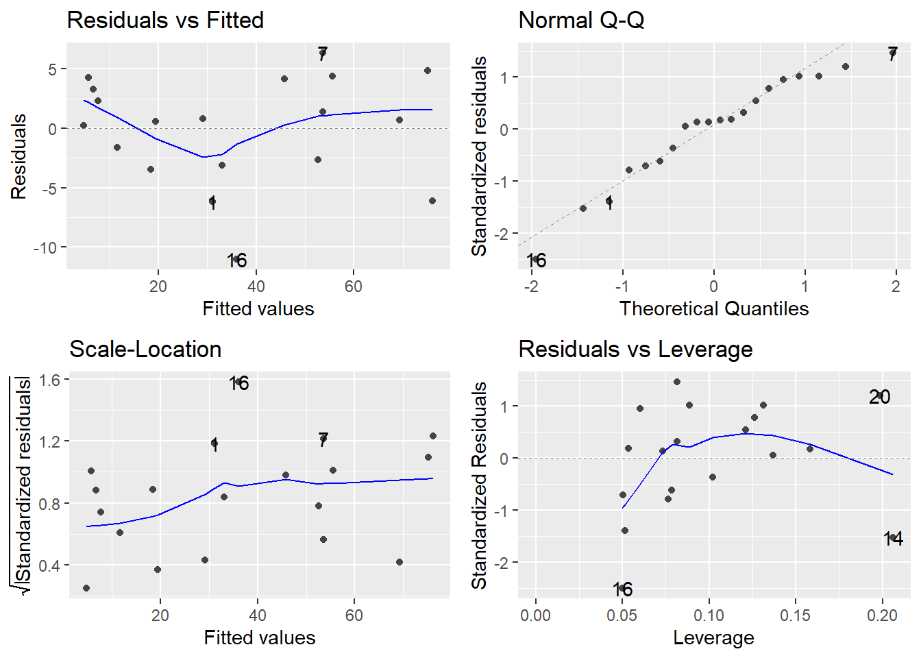
##
## [[3]]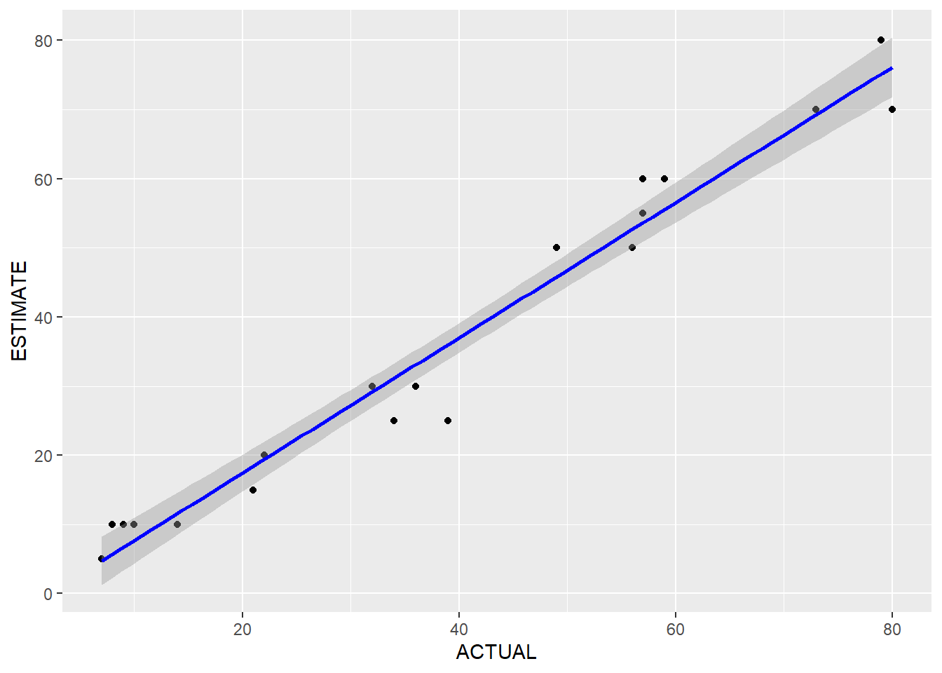
##
## --------------------------------------------------------
## a$TEST: POST2
## [[1]]
##
## Call:
## lm(formula = ESTIMATE ~ ACTUAL, data = df)
##
## Residuals:
##      Min       1Q   Median       3Q      Max
## -15.9575  -4.2873   0.8961   6.2328   9.6890
##
## Coefficients:
##              Estimate Std. Error t value Pr(>|t|)
## (Intercept) -11.40269    3.67614  -3.102  0.00615 **
## ACTUAL        1.21768    0.08178  14.889 1.46e-11 ***
## ---
## Signif. codes:  0 '***' 0.001 '**' 0.01 '*' 0.05 '.' 0.1 ' ' 1
##
## Residual standard error: 7.675 on 18 degrees of freedom
## Multiple R-squared:  0.9249, Adjusted R-squared:  0.9207
## F-statistic: 221.7 on 1 and 18 DF,  p-value: 1.46e-11
##
##
## [[2]]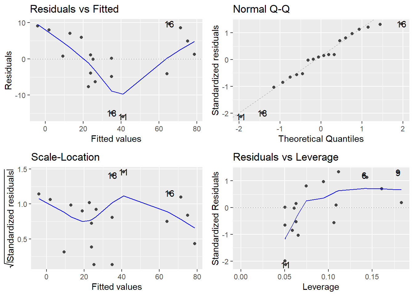
##
## [[3]]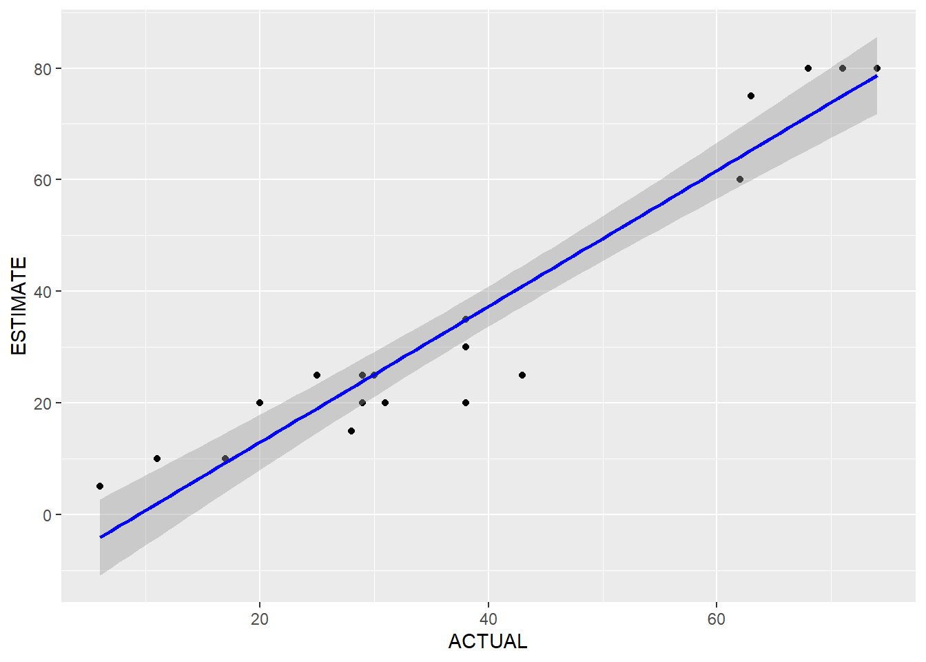
# Response: DIFF
diff_lm <- function(df){
    model <- lm(DIFF ~ ACTUAL, data = df)

    # fit plot
    fit_plot <- ggplot(data = df, aes(x = ACTUAL, y = DIFF)) +
        geom_point()+
        stat_smooth(method = "lm", col = "blue")

    return(list(summary(model), autoplot(model)))
}

by(a, a$TEST, diff_lm)
## a$TEST: BASELINE
## [[1]]
##
## Call:
## lm(formula = DIFF ~ ACTUAL, data = df)
##
## Residuals:
## Min 1Q Median 3Q Max
## -7.3419 -3.0730 0.3805 3.2750 6.3549
##
## Coefficients:
## Estimate Std. Error t value Pr(>|t|)
## (Intercept) -9.18368 1.81073 -5.072 7.95e-05 ***
## ACTUAL -0.01483 0.04030 -0.368 0.717
## ---
## Signif. codes: 0 '***' 0.001 '**' 0.01 '*' 0.05 '.' 0.1 ' ' 1
##
## Residual standard error: 4.264 on 18 degrees of freedom
## Multiple R-squared: 0.007463, Adjusted R-squared: -0.04768
## F-statistic: 0.1353 on 1 and 18 DF, p-value: 0.7172
##
##
## [[2]]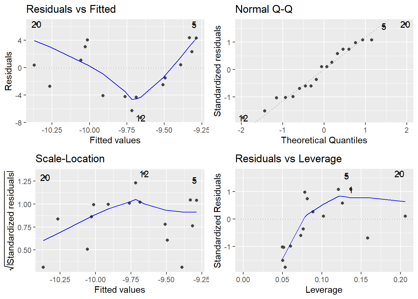
##
## --------------------------------------------------------
## a$TEST: POST1
## [[1]]
##
## Call:
## lm(formula = DIFF ~ ACTUAL, data = df)
##
## Residuals:
##      Min       1Q   Median       3Q      Max
## -11.0323  -2.7663   0.6561   3.5244   6.3667
##
## Coefficients:
##             Estimate Std. Error t value Pr(>|t|)
## (Intercept) -2.10325    1.91861  -1.096    0.287
## ACTUAL      -0.02217    0.04270  -0.519    0.610
##
## Residual standard error: 4.518 on 18 degrees of freedom
## Multiple R-squared:  0.01475,    Adjusted R-squared:  -0.03998
## F-statistic: 0.2695 on 1 and 18 DF,  p-value: 0.61
##
##
## [[2]]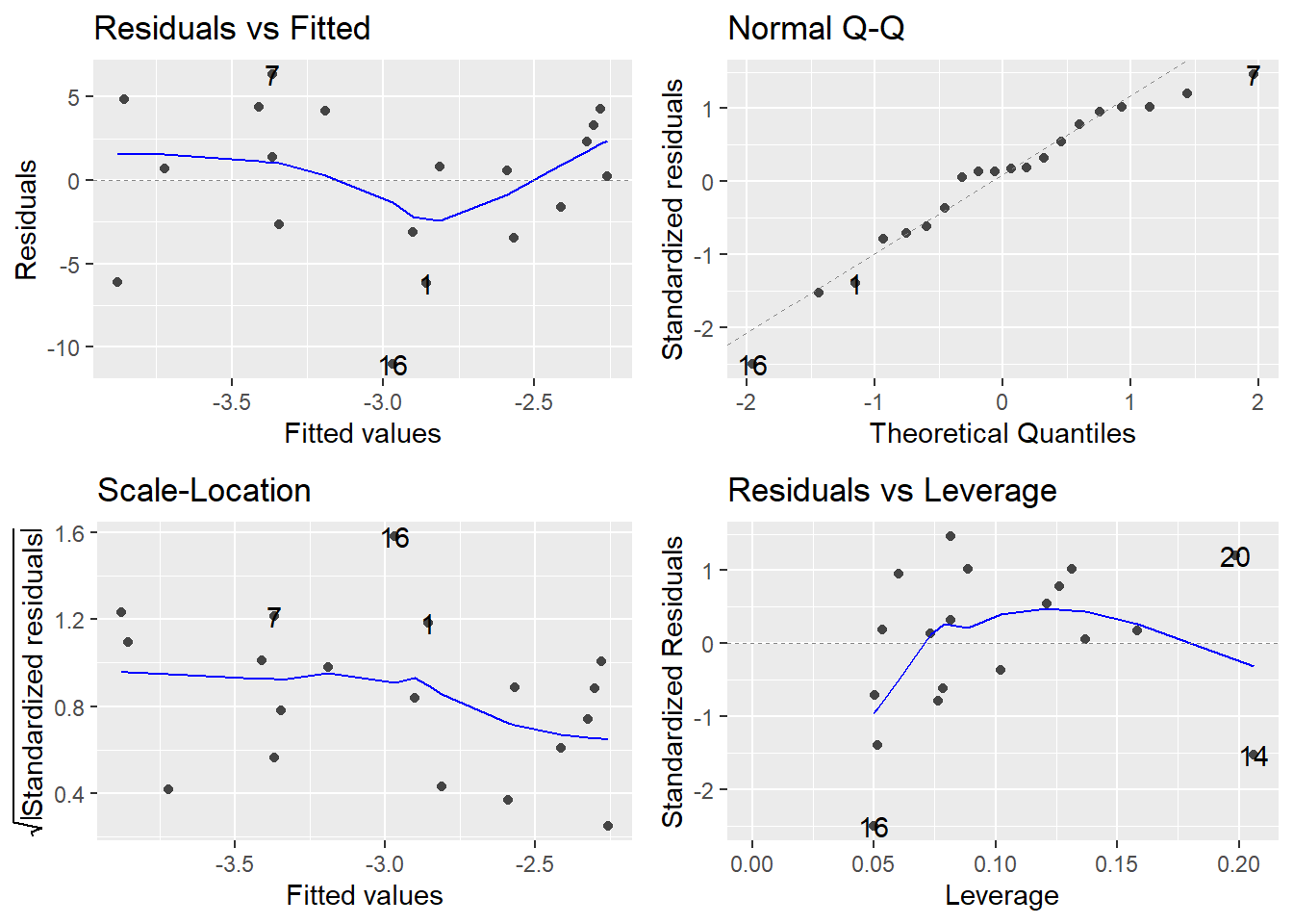
##
## --------------------------------------------------------
## a$TEST: POST2
## [[1]]
##
## Call:
## lm(formula = DIFF ~ ACTUAL, data = df)
##
## Residuals:
##      Min       1Q   Median       3Q      Max
## -15.9575  -4.2873   0.8961   6.2328   9.6890
##
## Coefficients:
##              Estimate Std. Error t value Pr(>|t|)
## (Intercept) -11.40269    3.67614  -3.102  0.00615 **
## ACTUAL        0.21768    0.08178   2.662  0.01589 *
## ---
## Signif. codes:  0 '***' 0.001 '**' 0.01 '*' 0.05 '.' 0.1 ' ' 1
##
## Residual standard error: 7.675 on 18 degrees of freedom
## Multiple R-squared:  0.2824, Adjusted R-squared:  0.2426
## F-statistic: 7.084 on 1 and 18 DF,  p-value: 0.01589
##
##
## [[2]]